Another important type of latent variable models are latent growth curve models. Growth modeling is often used to analyze longitudinal or developmental data. In this type of data, an outcome measure is measured on several occasions, and we want to study the change over time. In many cases, the trajectory over time can be modeled as a simple linear or quadratic curve. Random effects are used to capture individual differences. The random effects are conveniently represented by (continuous) latent variables, often called growth factors. In the example below, we use an artifical dataset called Demo.growth where a score (say, a standardized score on a reading ability scale) is measured on 4 time points. To fit a linear growth model for these four time points, we need to specify a model with two latent variables: a random intercept, and a random slope:
# linear growth model with 4 timepoints
# intercept and slope with fixed coefficients
 i =~ 1*t1 + 1*t2 + 1*t3 + 1*t4
 s =~ 0*t1 + 1*t2 + 2*t3 + 3*t4
In this model, we have fixed all the coefficients of the growth functions. If i and s are the only ‘latent variables’ in the model, we can use the growth() function to fit this model:
model <-' i =~ 1*t1 + 1*t2 + 1*t3 + 1*t4 s =~ 0*t1 + 1*t2 + 2*t3 + 3*t4 'fit <-growth(model, data=Demo.growth)summary(fit)
lavaan 0.6-21 ended normally after 29 iterations

  Estimator                                         ML
  Optimization method                           NLMINB
  Number of model parameters                         9

  Number of observations                           400

Model Test User Model:

  Test statistic                                 8.069
  Degrees of freedom                                 5
  P-value (Chi-square)                           0.152

Parameter Estimates:

  Standard errors                             Standard
  Information                                 Expected
  Information saturated (h1) model          Structured

Latent Variables:
                   Estimate  Std.Err  z-value  P(>|z|)
  i =~
    t1                1.000
    t2                1.000
    t3                1.000
    t4                1.000
  s =~
    t1                0.000
    t2                1.000
    t3                2.000
    t4                3.000

Covariances:
                   Estimate  Std.Err  z-value  P(>|z|)
  i ~~
    s                 0.618    0.071    8.686    0.000

Intercepts:
                   Estimate  Std.Err  z-value  P(>|z|)
    i                 0.615    0.077    8.007    0.000
    s                 1.006    0.042   24.076    0.000

Variances:
                   Estimate  Std.Err  z-value  P(>|z|)
   .t1                0.595    0.086    6.944    0.000
   .t2                0.676    0.061   11.061    0.000
   .t3                0.635    0.072    8.761    0.000
   .t4                0.508    0.124    4.090    0.000
    i                 1.932    0.173   11.194    0.000
    s                 0.587    0.052   11.336    0.000
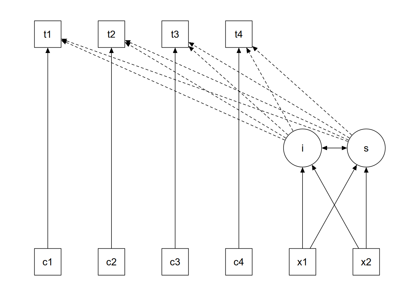
Technically, the growth() function is almost identical to the sem() function. But a mean structure is automatically assumed, and the observed intercepts are fixed to zero by default, while the latent variable intercepts/means are freely estimated. A slightly more complex model adds two regressors (x1 and x2) that influence the latent growth factors. In addition, a time-varying covariate c that influences the outcome measure at the four time points has been added to the model. A graphical representation of this model is presented below.
A growth curve examples
The complete R code needed to specify and fit this linear growth model with a time-varying covariate is given below:
# a linear growth model with a time-varying covariatemodel <-' # intercept and slope with fixed coefficients i =~ 1*t1 + 1*t2 + 1*t3 + 1*t4 s =~ 0*t1 + 1*t2 + 2*t3 + 3*t4 # regressions i ~ x1 + x2 s ~ x1 + x2 # time-varying covariates t1 ~ c1 t2 ~ c2 t3 ~ c3 t4 ~ c4'fit <-growth(model, data = Demo.growth)summary(fit)